
HWT/DTC 2011 Evaluation - Traditional Methods
Traditional Verification Methods
Statistics for dichotomous (2-category) variables
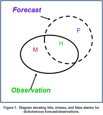
For dichotomous variables (e.g., precipitation amount above or below a threshold) on a grid, typically the forecasts are evaluated using a diagram like the one shown in Fig. 1. In this diagram, the area “H” represents the intersection between the forecast and observed areas, or the area of Hits; “M” represents the observed area that was missed by the forecast area, or the “Misses”; and “F” represents the part of the forecast that did not overlap an area of observed precipitation, or the “False Alarm” area. A fourth area is the area outside both the forecast and observed regions, which is often called the area of “Correct Nulls” or “Correct Rejections”.
This situation can also be represented in a “contingency table” like the one shown in Table 1. In this table the entries in each “cell” represent the counts of hit, misses, false alarms, and correct rejections. The counts in this table can be used to compute a variety of traditional verification measures, described in the following sub-sections.
Table 1. Contingency table illustrating the counts used in verification statistics for dichotomous (e.g., Yes/No) forecasts and observations. The values in parentheses illustrate the combination of forecast value (first digit) and observed value. For example, YN signifies a Yes forecast and and a No observation.
Forecast |
Observed |
||
Yes |
No |
|
|
Yes |
Hits (YY) |
False alarms (YN) |
YY + YN |
No |
Misses (NY) |
Correct rejections (NN) |
NY + NN |
|
YY + NY |
YN + NN |
Total = YY + YN + NY + NN |
Base rate
![]()
Also known as sample climatology or observed relative frequency of the event.
Answers the question:What is the relative frequency of occurrence of the Yes event?
Range: 0 to 1.
Characteristics: Only depends on the observations. For convective weather can give an indication of how “active” a day is.
Probability of detection (POD)
![]()
Also known as Hit Rate.
Answers the question: What fraction of the observed Yes events was correctly forecasted?
Range: 0 to 1. Perfect score: 1.
Characteristics: Sensitive to hits, but ignores false alarms. Good for rare events. Can be artificially improved by issuing more Yes forecasts to increase the number of hits. Should be used in conjunction with the false alarm ratio (below) or at least one other dichotomous verification measure. POD is an important component of the Relative Operating Characteristic (ROC) used widely for evaluation of probabilistic forecasts.
False alarm ratio (FAR)
![]()
Answers the question: What fraction of the predicted "yes" events did not occur (i.e., were false alarms)?
Range: 0 to 1. Perfect score: 0.
Characteristics: Sensitive to false alarms, but ignores misses. Very sensitive to the climatological frequency of the event. Should be used in conjunction with the probability of detection (above). FAR is an important component of the Relative Operating Characteristic (ROC) used widely for evaluation of probabilistic forecasts.
Bias
![]()
Also known as Frequency Bias.
Answers the question: How similar were the frequencies of Yes forecasts and Yes observations?
Range: 0 to infinity. Perfect score: 1.
Characteristics: Measures the ratio of the frequency of forecast events to the frequency of observed events. Indicates whether the forecast system has a tendency to underforecast (Bias < 1) or overforecast (Bias > 1) events. Does not measure how well the forecast gridpoints correspond to the observed gridpoints, only measures overall relative frequencies. Can be difficult to interpret when number of Yes forecasts is much larger than number of Yes observations.
Critical Success Index (CSI)
Also known as Threat Score (TS).
![]()
Answers the question: How well did the forecast "yes" events correspond to the observed "yes" events?
Range: 0 to 1, 0 indicates no skill. Perfect score: 1.
Characteristics: Measures the fraction of observed and/or forecast events that were correctly predicted. It can be thought of as the accuracy when correct negatives have been removed from consideration. That is, CSI is only concerned with forecasts that are important (i.e., assuming that the correct rejections are not important). Sensitive to hits; penalizes both misses and false alarms. Does not distinguish the source of forecast error. Depends on climatological frequency of events (poorer scores for rarer events) since some hits can occur purely due to random chance. Non-linear function of POD and FAR. Should be used in combination with other contingency table statistics (e.g., Bias, POD, FAR).
Gilbert Skill Score (GSS)
Also commonly known as Equitable Threat Score (ETS).
![]()
where
![]()
Answers the question: How well did the forecast "yes" events correspond to the observed "yes" events (accounting for hits that would be expected by chance)?
Range: -1/3 to 1; 0 indicates no skill. Perfect score: 1.
Characteristics: Measures the fraction of observed and/or forecast events that were correctly predicted, adjusted for the frequency of hits that would be expected to occur simply by random chance (for example, it is easier to correctly forecast rain occurrence in a wet climate than in a dry climate). The GSS (ETS) is often used in the verification of rainfall in NWP models because its "equitability" allows scores to be compared more fairly across different regimes; however it is not truly equitable. Sensitive to hits. Because it penalizes both misses and false alarms in the same way, it does not distinguish the source of forecast error. Should be used in combination with at least one other contingency table statistic (e.g., Bias).
Statistics for Continuous Variable
Statistics for continuous forecasts and observations
For this category of statistical measures, the grids of forecast and observed values – such as precipitation or reflectivity – are overlain on each other, and error values are computed. The grid of error values is summarized by accumulating values at all of the grid points and used to compute measures such as mean error and root mean squared error.
These statistics are defined in the sub-sections below. In the equations in these sections, fisignifies the forecast value at gridpoint i, oi represents the observed value at gridpoint i, and N is the total number of gridpoints.
Mean error (ME)
![]()
Also called the (additive) Bias.
Answers the question: What is the average forecast error?
Range: minus infinity to infinity. Perfect score: 0.
Characteristics: Simple, familiar. Measures systematic error. Does not measure the magnitude of the errors. Does not measure the correspondence between forecasts and observations; it is possible to get a perfect ME score for a bad forecast if there are compensating errors.
Pearson Correlation Coefficient (r)

where![]() is the average forecast value
and
is the average forecast value
and ![]() is the average observed
value.
is the average observed
value.
Also called the linear correlation coefficient.
Answers the question: What is the linear association between the forecasts and observations?
Range: -1 to 1. Perfect score: 1
Characteristics: r can range between -1 and 1; a value of 1 indicates perfect correlation and a value of -1 indicates perfect negative correlation. A value of 0 indicates that the forecasts and observations are not correlated. The correlation does not take into account the mean error, or additive bias; it only considers linear association.
Mean squared error (MSE) and root-mean squared error (RMSE)
![]()
![]()
MSE can be re-written as
![]() ,
,
where ![]() is the average forecast value,
is the average forecast value, ![]() is the average observed
value, sf is the standard deviation of the forecast values, so is the standard deviation of the observed values, and rfois
the correlation between the forecast and observed values. Note that
is the average observed
value, sf is the standard deviation of the forecast values, so is the standard deviation of the observed values, and rfois
the correlation between the forecast and observed values. Note that ![]() and
and ![]() is the estimated variance of
the error,
is the estimated variance of
the error,![]() . Thus,
. Thus,![]() . To
understand the behavior of MSE, it is important to examine both of these terms of MSE, rather than examining MSE alone.
Moreover, MSE can be strongly influenced by ME, as shown by this
decomposition.
. To
understand the behavior of MSE, it is important to examine both of these terms of MSE, rather than examining MSE alone.
Moreover, MSE can be strongly influenced by ME, as shown by this
decomposition.
The standard deviation of the
error, sf-o, is simply ![]() .
.
Note that the standard deviation of the error (ESTDEV) is sometimes called the “Bias-corrected MSE” (BCMSE) because it removes the effect of overall bias from the forecast-observation squared differences.
Answers the question: What is the average magnitude of the forecast errors?
Range: 0 to infinity. Perfect score: 0.
Characteristics: Simple, familiar. Measures "average"
error, weighted according to the square of the error. Does not indicate the
direction of the deviations. The RMSE puts greater influence on large errors
than smaller errors, which may be a good thing if large errors are especially
undesirable, but may also encourage conservative forecasting.